Speed Control Of A Three Phase Induction Motor Using Field Oriented Control
Eng. Mohamed Hussein, Dr. Mahfooz E. Shalaby, Dr. Hamdy A.M. Shatla, Dr. Amr Refky,
Dept. of Electrical Engineering Al-Azhar University Cairo, Egypt Eng_mo.hussein@yahoo.com
Abstract—Induction Motors are rugged, robust and widely used in industrial applications. Field oriented control (FOC) or Vector control is an efficient method to control either the speed or the torque or both of the three phase Induction motor. FOC converts the complex stator currents into two orthogonal components, one of which is responsible for speed control, and the other for the electromagnetic torque control, similar to DC machines. FOC has greater stability and capable of fast torque response and accurate speed control. This research explains the concept of FOC and its simulation rather than experimental implementation using Matlab simulink and MexBios softwares.
Keywords— Three phase Induction Motor; Scaler Control; Simulink program; MexBios software; Field oriented control (FOC); Field oriented control semulation.
I. INTRODUCTION
Induction motors are the preferred choice for industrial applications due to their rugged construction, maintenance free and development in power electronics, which leads to easy control of motor speed.
The three-phase Induction Motors speed is:

where;
fs: Supply frequency in Hz p: Number of pole pairs of stator
S: Slip between of rotating field and mechanical speeds
The speed of three phase Induction motor can be controlled by varying the frequency of the applied stator voltage via scalar control or vector control methods.
II. FIELD ORIENTED CONTROL
Field oriented control or offers more precise control of ac motors compared to scalar control. FOC is therefore used in high performance drives where oscillations in air gap flux linkages are intolerable, e.g. robotic actuators, centrifuges etc. In Field oriented control method, the components of the motor stator currents are represented by two orthogonal components in a rotating reference frame. In a special reference frame, the expression for the electromagnetic torque of the smooth-air-gap machine is similar to the expression for the torque of the separately excited DC machine. The control is normally performed in a reference frame aligned to the rotor flux space vector.
The field oriented algorithm controls the components of the motor stator currents, represented by a vector, in a rotating reference frame d, q aligned with the rotor flux and perpendicular directions. The Clarke transformation converts three-phase currents ia, ib and ic into two-phase orthogonal stator currents: ia and ib. These two currents in the fixed coordinate stator phase are transformed to the id and iq currents components in the d, q reference frame using Park transformation.
The stator variables are translated into a flux model which is compared with a required reference values and then is tuned by PI controllers. After a back transformation from field to stator coordinates, the output voltage will be impressed to the machine with Pulse Width Modulation (PWM) technique [2, 3 and 4].

Fig. 1. Stator currents in the d, q rotating reference frame
where;
ia , ib , ic : Three-phase stator currents id : Direct current iq : Quadrature current iα , iβ : Two-phase orthogonal current θ : The phase frame rotation angle
A. Mathematical Clarke transform
The mathematical Clarke transformation converts a three-phase system to a two-phase orthogonal system is obtained from:
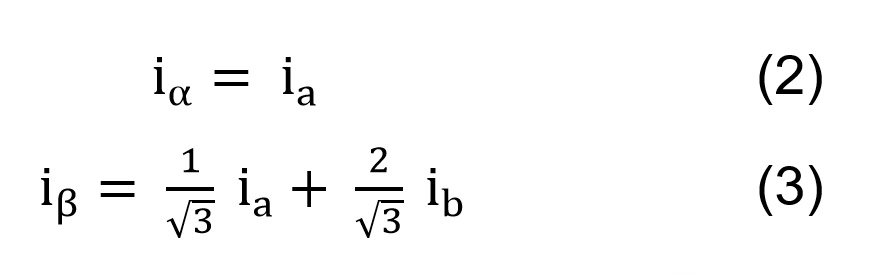
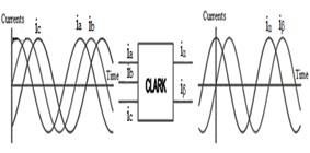
Fig. 2. Direct Clark Transform
B. Mathematical Park transform
The two phase components in the α, β frame representation calculated using Clarke transformation are then fed to a vector rotation block where it is rotated over a flux angle ρ to follow the frame d, q coincides to the rotor flux [2, 3 and 4].
The rotation over a flux angle ρ is achieved according to the formulae:


Fig.3. Direct Park Transform
C. Mathematical Inverse Park and Clarke transforms Transformation uses the Inverse Clarke transformation, Figure 4.The vectors in the d, q frame are transformed from d, q frame to the two phases α, β frame representation calculated with rotation over a flux angle ρ according to the formulae:
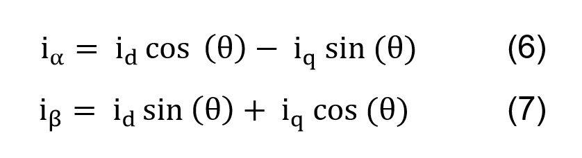

Fig. 4. Inverse Park Transform
The modification from a two-phase orthogonal α, β frame to a three-phase system is done using the equations:
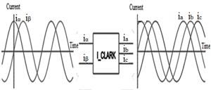
Fig. 5. Inverse Clarke Transform
III. SIMULINK PROGRAM
Simulink is a software add-on to MATLAB which is a mathematical tool that enables to simulate model, and analyze systems whose outputs change over time. Such systems are often referred to as dynamic systems.
S-functions (system-functions) provide a powerful mechanism for extending the capabilities of Simulink to allow addition new blocks to Simulink models [5].
A. Simulation of Vector Control of Induction Motor using Simulink program
Vector Control of three phase Induction Motor is simulated by the block diagram and S-Function as shown in Figures. 6 and 7 with following components:
- Three phase Induction Motor
- Clarke and Park transforms
- Id_PI controller 4- Iq_PI controller
- Inverse Park and Clarke transforms
- Plus width modulation (PWM)
- Three phase Inverter 8- Speed PI controller
The simulation of the Motor starts at No load and when the Motor reaches the steady state speed, there will be two case studies of simulation:
- Rotating the motor in the reverse direction by inversing the sign of quadrature current (Iq) with no load.
- Increasing the load torque (Tm).
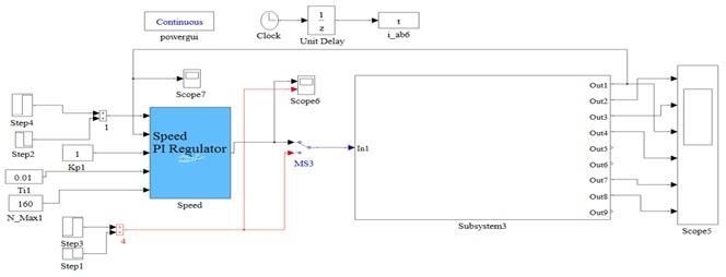
Fig. 6. Field oriented control for three phase Induction Motor schematic diagram in Simulink
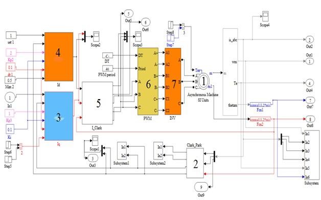
Fig. 7. Matlab Subsystem schematic diagram
B. Rotating the motor in the reverse direction
The motor starts with no load, the three phase
currents (ia, ib, ic) will start with large values (Istart) and they will have some distortions until the motor reaches it's no load speed. When the motor reaches its rated speed and its rated three phase currents, the motor continues running with no load for 0.5 seconds until we inverse the sign of quadrature current (Iq).
So, the quadrature current (Iq) reaches its peak value with negative sign then falls down to be close zero value because the motor runs with no load and the Direct current continue with its positive value as shown in Figure 8.
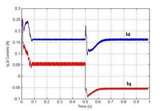
Fig. 8. Two phase currents VS Time
When the motor starts, the electromagnetic torque increases to reach the peak value, then falls down to be close zero value because the motor runs with no load. After Inversing the sign of quadrature current (Iq), the torque inverses its sign to reach the peak value and also falls down to be close zero value but with negative sign as shown in Figure 9.

Fig. 9. Motor electromagnetic torque VS Time
When we inverse the sign of quadrature current (Iq) the motor will rotate in the reverse direction because the motor torque will inverse it's direction and the stator currents (ia, ib, ic) will be reflected from (R S T) to (S T R) as shown in Figure 10.
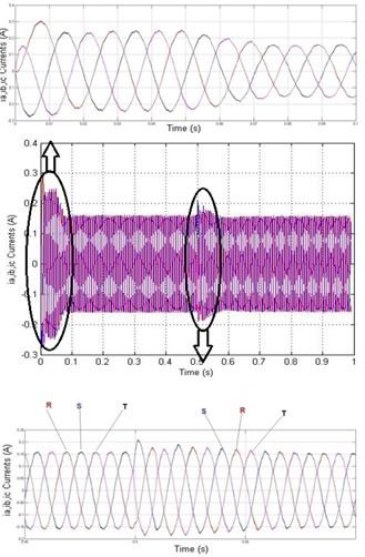
Fig. 10. Three phase (ia, ib, ic) starting currents and after reflected from (R S T) to (S T R)
The motor speed will decrease to zero value, then the motor will reverse its rotation direction and will continue running at the reverse direction to reach the rated speed as shown in Figure 11.

Fig. 11. Speed VS Time
When the motor starts with no load, the value of Theta increases slowly. After the motor reaches its rated speed, the value of Theta continues increasing with fast regular values. After Inversing the sign of quadrature current (Iq), the value of Theta starts decreasing and after the motor reaches the rated speed in the reverse direction, the value of Theta will decrease regularly. The simulation uses a function block to make the value of Theta increases to reach (2*pi) then falls down to zero and so on. At the reverse direction, the value of Theta decreases to reach zero value then rises up to (2*pi) and so on as shown in Figure 12.

Fig. 12. Theta VS Time
C. Increasing the load torque using Current control
In this simulation the motor starts at No load and continue running with no load for (0.5 seconds) and after that we will suddenly increase the load torque (Tm), So, the three phase currents (ia, ib, ic) will increase to cover this load, The (Iq PI controller) will increase the value of quadrature current (Iq) but the value of direct current (Id) will not be affected because the direct current responsible only for the magnetization and the quadrature current (Iq) responsible for the torque as shown in Figure 13.
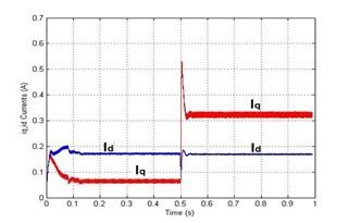
Fig. 13. Two phase currents/Time when increasing the torque
We note that when the motor starts, the mechanical torque increases to reach the peak value and falls down to be close zero value because the motor running with no load. After the load increases, the motor output torque will increase to cover this load as shown in Figure 14.

Fig. 14. Torque VS Time at increasing the load
When we use Current control only the motor speed will decrease according to the increase of the load but the controller will control the output speed to make the decrease of the speed better p.u. values as shown in Figure 15.

Fig. 15. Speed VS Time at increasing the load torque using
Current control only
D. Increasing the load torque using Speed and Current control
In this simulation the motor starts at No load and after the motor reaches its rated speed the simulation will increase the load torque suddenly but will increase speed PI_controller to control the speed.
The speed PI_controller will increase speed
PI_controller to control the speed.
The speed PI_controller will cover the decrease of the speed to fix the speed at the set point of the speed PI controller we note that when we compare between Figures 15 and 16.
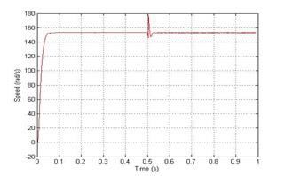
Fig. 16. Speed VS Time at increasing the load torque using Speed and Current control
IV. MEXBIOS SOFTWARE
MexBios software is a mathematical tool used to simulate vector control of three phase Induction motor. MexBios software has a very important feature, that it can simulate the program before loading it to Microcontroller, so the results can be expected by simulation before running the real Motor. MexBios program will simulate Vector Control of Induction Motor and the same program will be loaded to the
Microcontroller [6].
A. Simulation of Vector Control of Induction Motor using MexBios program
The Simulation uses MexBios software to simulate Sensor Less Vector Control of two phase Induction Motor by simulating all components for the following schematic diagram as shown in Figure 17:

Fig. 17. Schematic diagram of control blocks
Schematic diagram for control blocks contains:
1- GUI (Graphical User Interface) which contains:
- RADIO IN selector to select between Feedback from Motor Model or from real Motor
- Reset Start / Stop Switch to reset all feedback signals
- CLARK transform.
Drivers ADC QEP Formula shown in Figure 18 contains:
- GIPO inputs & outputs.
- QEP block process the Encoder signals

Fig. 18. Drivers ADC QEP Formula internal details
Current Loop Formula contains the following as shown in Figure 19:
- Current model rotor AD
- PID controller duty cycle of keys Inverter required for PWM.
- PARK & IPARK transforms
- A_MUX switches
- Seven_DQ block to generate a corresponding

Fig. 19. Drivers ADC QEP Formula internal details
When the positive value of quadrature current, the motor Speed starts from zero and increases fast (only one second) to reach the peak value (0.97 PU), these value mean that the motor runs at No load Speed. After the Motor reaches No load Speed, it will continue as shown in Figure 20.
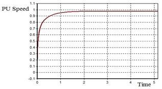
Fig.20. Speed Time response
When the motor starts, the starting Iq, Id currents reach their peak values and starting to decrease to reach their No load values as shown in Figure 21 a and After the Motor reaches No load Speed, direct and quadrature currents will continue at their
No load values as shown in Figure 21 b.

Fig. 21.a) Iq, Id starting values b). Iq, Id No load values
Since the Motor starts with Sensorless control, the value of Theta will start with a lot of disturbances for only few milliseconds until the Motor feedback signals return to the control circuits as shown in Figure 22 a and Fig 22 b, the same also happens with real work as in Figures 29 and 30.
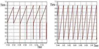
Fig. 22 a.) Theta starting value b.) Theta after few milliseconds

Fig. 23: Speed curve in PU with negative quadrature current
When the motor starts, the starting Iq, Id currents reache their negative peak values and starting to increase to reach their negative No load values as shown in Figure 24 a. After the Motor reaches No load Speed, Iq, Id currents will continue at their negative No load values as shown in Figure 24 b.

Fig. 24 a): Tow phase current starting values with negative load b): Tow phase current No values with negative quadrature current quadrature current
The value of Theta will start from zero and jump to one. Theta starts to decrease to reach to zero and jump again to one and so on. Because the Motor starts with Sensor less control, the value of Theta will start with a lot of disturbances for only few milliseconds until the Motor feedback signals return to the control circuits as shown in Figure 25 a and Figure 25 b.
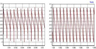
Fig. 25 a): Theta starting values with negative quadrature b): Theta after few milliseconds with negative quadrature
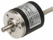
Fig.26: Incremental shaft encoder BDK 05A 1024 PPR
The position information is delivered using a series of pulses – usually in phase quadrature, so that direction of travel can be determined. These are usually referred to as A/B pulses as shown in Figure 27. A separate pulse train, typically referred to as the N reference, provides one pulse per revolution to act as a reference mark [7].

Fig. 27: Schematic of an incremental optical sensor with a reference pulse

Fig. 28: Connection between MCB-2 Kit and Laptop using mZdsp 2812 Kit and XDS 100V2 emulator
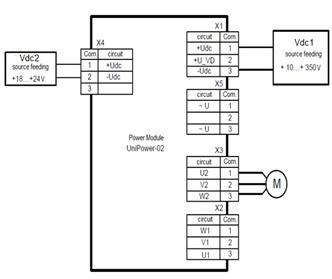
Fig. 29: Connection diagram
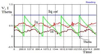

Fig. 31: Output curves at Iq ref. = -1